Machine Cycle Analysis: Detecting Tool Wear, Quality Issues, and Downtime Proactively

Every tool in a CNC machine leaves a data profile on every cycle. Data profiles include things such as: spindle loads, axis loads, servo temperatures, bearing temperatures, offsets, alignments, and more. Machine profile deviation detection learns what a normal profile looks like for each tool and flags the cycles that stray from it. Those deviations are early warnings of the two most expensive problems in machining: parts going out of tolerance, and machines heading for unplanned downtime.

By the time anyone notices, it is already expensive

Most CNC operations find a bad part the same way: a feature measures out of tolerance at the inline gauge, the CMM or final inspection. By then the spindle has already cut that part, and usually the next several. If the cause is a chipped insert, a loose fixture or a crashed offset, every part since it started is suspect.

Downtime arrives the same way. A worn tool keeps cutting until it breaks, sometimes taking the part, the holder or the spindle with it. A spindle bearing or axis drive degrades for weeks, and the first sign anyone sees is an alarm and a stopped machine. Then the cost is the lost spindle hours, the rush for parts and service, and every job queued behind that machine.

In both cases the machine knew earlier. A wearing tool, a part sitting slightly off its datum, or a spindle or axis that is starting to degrade all change the spindle and axis loads. Those changes show up long before they appear on a feature or as an alarm. The loads are already being collected. What has been missing is a way to read them per tool, per cycle, against what normal looks like for that exact cut.

Downtime and quality issues are killing capacity

Most factories plan capacity around the cycle times on the router, but the time actually lost sits off that schedule. A suspect batch means stopping the machine, sorting parts, re-measuring and re-running. 

A tool failure means pulling the part, inspecting the spindle, finding a replacement and re-proving the program. Each event looks small and nobody tracks it, but together they quietly take hours out of every shift. The machine sits idle while someone investigates. 

The robot or pallet system that was supposed to run lights-out waits on a person to clear the fault. Your most experienced machinists and engineers spend the day fighting fires instead of setting up new jobs, improving processes or running more spindles. The result is expensive equipment, automation and skilled people that look fully booked on paper but are badly underused in practice. That gap is capacity you’ve already paid for and can’t get to. 

Process control must be fully automated to gain capacity

People can’t solve this by watching machine signals and sifting data. Every cycle produces tens of thousands of readings across every tool and axis, far more than anyone can review, and sampling inspection only confirms what has already gone wrong. 

The system has to understand the data in context: the program, the tool, the operation, and what normal looks like for that cut. Then it has to act on its own. It notifies operations or engineers, adjusts an offset, calls a tool change, stops the machine or quarantines a suspect part before the problem costs you parts or spindle hours.

Why analyze machine cycle profiles?

The machine profile is the only record that exists for every cycle of every tool, names the tool that was in cut, and is available before the part reaches the gauge or the machine stops. Every other approach a plant typically relies on gives up at least one of those.

Approach	What it tells you	What it misses
Inspection alone	Whether a measured feature is in tolerance	Only parts that get measured, and only after they are cut. It names a feature, not the tool or the moment that caused it
Tool life counters	When a tool has done its planned number of parts or minutes	Whether the tool is actually worn. Tools get changed too early, which wastes life, or too late, which makes scrap or breaks the tool
A fixed load limit per tool	That load crossed one threshold somewhere in the cycle	Everything below the threshold. A load that is normal while roughing can be a problem while finishing, and a single limit cannot tell them apart
Machine profile analysis	How each cycle compares with that tool’s normal cut, point by point, and whether the difference hurt the part	It depends on load data being collected per tool, and on inspection results being recorded against the part

The point-by-point comparison is what makes the difference. A cut is a sequence: entry, engagement, peak load, finishing passes, exit. Comparing each point with the same point in a normal cycle catches a change in one part of the cut that a whole-cycle average or a single threshold would never see.

In the Flexxbotics Platform, this granular type of data collection, contextualization, and process characterization is possible. No extra hardware is needed. The machining data come from the CNC controller that is already running the program.

Learning what a normal cycle looks like for every tool

The analysis works one tool signal at a time, for example: Tool 5’s Z-axis load, the spindle load while Tool 12 is in cut, and so on. This is foundational to how data is collected and contextualized. Each signal is a curve that rises and falls as the tool enters the material, works through the toolpath and retracts. For a given tool on a given program, that curve should look much the same every time.

Building the reference takes four steps:

1. Split the stream into cycles. Readings are grouped by the part they were taken on, so each cycle is one tool’s pass over one part. Fragments where the tool was barely in cut are set aside.
2. Line the cycles up. No two cycles have exactly the same number of samples or the same timing. Each is stretched onto a common timeline, so the start of the cut is compared with the start of the cut and the peak of the cut with the peak of the cut.
3. Pick the cycles that define normal. By default the analysis looks for the cycles that most resemble each other anywhere in the time window, rather than assuming the first ones were good. That way, a tool that was already wearing when the window opened does not become the definition of normal.
4. Build the reference profile. From those cycles it computes a typical curve and a band around it, the range of a healthy cycle stays inside at each point of the cut. The band uses a median-based measure of spread, so a handful of odd cycles cannot widen it to the point where nothing looks unusual.

Prescriptive optimization is the capability within the Flexxbotics Platform that automates this analysis. 

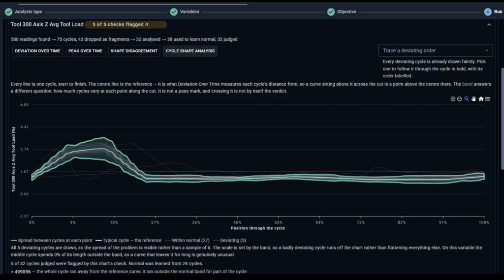
Each line represents a single cycle that has run on a single part. The X-Axis represents the percentage of the cycle that has been completed. The center dark line is the “normal” profile of the machining for all the cycles and is determined by the cycles that all agree with each other. The top and bottom lines represent the amount of variation at each portion of the cycle. 

The result is a reference profile for every tool signal on every part and operation: what this cut normally looks like and how much it normally varies. An engineer can review it and accept it as the known-good characterization. From then on, every later run is judged against that accepted reference rather than relearning normal from whatever happens to be in the window.

Spotting the cycles that deviate

Every cycle is compared with its tool’s reference profile and scored in several independent ways. Each way catches a different kind of problem:

• Level. Did the whole cycle run higher or lower than the reference? Example: a tool that is dulling typically pulls more load throughout the cut.
• Peak. Was the peak load of the cut outside its normal range? Many crashes, chips and entry problems show up here first.
• Time outside the band. Did the cycle spend a meaningful share of the cut outside the normal band, rather than just touching it?
• Disagreement. Did the cycle run above the reference in some places and below it in others? Its average can look perfect while the cut itself is not.
• Shape. Did the curve come out a different shape, such as a step that moved, a dwell that appeared, or a pass that is missing?

A cycle is flagged when one of these scores falls outside limits learned from the clean reference cycles. Every flag comes with the reason in plain words, for example “its peak reading was outside the normal range” or “the whole cycle ran higher than the reference curve”. The flagged points are marked on the charts, so you see which cycles were flagged and why.

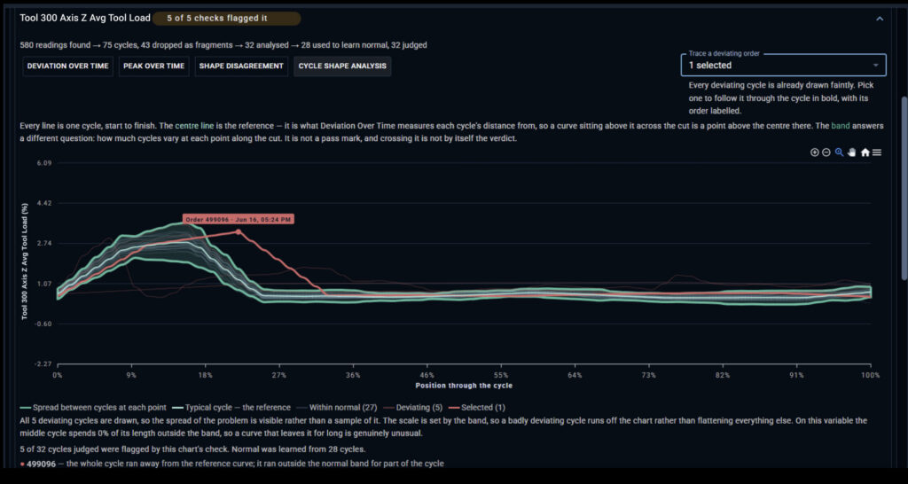
The red line represents a cycle that fell outside the “normal” profile of the cut indicating that something in the process changed or drifted causing this cutting process to look different than normal. 

The most valuable signal is often not a single bad cycle but slow drift: a profile that climbs a little with every part. The analysis searches the run for the stretch where the level changes the most and tests whether that change is real. The test accounts for how many stretches it searched, so it does not report a trend in what is only noise. When a drift is real, it reports the production orders where the drift started and ended, plus the size of the change.

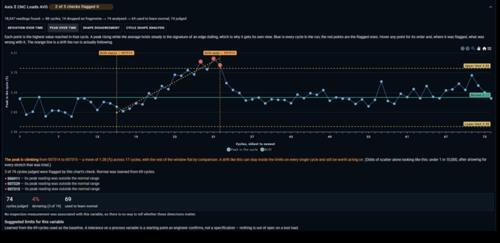
Each point on this graph represents the total amount of deviation from the “normal” curve for each cycle that was run. It looks at the deviation from cycle to cycle and can detect trends on it. This is an indicator of a machine health issue that is showing an increasing amount of deviation in the normal cutting profile from cycle to cycle. This analysis is used to establish limits and average operating conditions and can be used to indicate that maintenance on this particular tool or axis is needed. 

Does the deviation matter? Check against inspection

A deviating cycle is only worth acting on if it changes the part. So each tool signal can be paired with the inspection measurement it affects, such as the bore diameter that Tool 5 finishes or the face height that Tool 12 cuts. Every flagged cycle is then checked against the measured result of the exact part it cut.

The match is made part by part where the inspection data allows it, and by production order where it does not. Each matched part falls into one of four groups:

	Measured in tolerance	Measured out of tolerance
Cycle flagged	False alarm	Caught
Cycle normal	Correctly quiet	Missed

From those four counts the analysis reports three numbers an engineer can act on:

• Flagged that were bad. Of the cycles it flagged, the share that produced an out-of-tolerance part. This is how much to trust an alert.
• Quiet that were good. Of the cycles it passed, the share that produced a good part. This is how much to trust silence.
• Bad parts caught. Of the parts that went out of tolerance, the share whose cycle was flagged beforehand. This is how much of the scrap the signal would have warned about.

This is what separates useful signals from noise. Some tools deviate all the time with no effect on the part, and those should not page anyone. Others deviate rarely, and when they do the part is bad. Inspection data tells you which is which, so attention goes to the tools whose behaviour actually decides part quality.

What it catches in machining operations

Different failures leave different marks in the loads. That is what lets the analysis point at a likely cause instead of just raising an alarm.

Issue	What it typically looks like in the loads	What you do with it
Tool wear	Level and peak climb slowly over many parts, and a drift is reported with start and end orders	Plan the tool change from the drift instead of waiting for a part to fail
Tool change timing	Inspection results start failing once the load passes a certain level	Change the tool before it reaches that load, which sets the change point by part quality rather than a fixed count
Chipped or broken tool	One cycle, or a sudden run of cycles, jumps in peak or level	Stop and inspect the tool, then quarantine parts from the first flagged cycle onward
Setup or offset error	A step change in level or shape that starts at one production order, often right after a changeover, across several tools	Go back to the setup at that order: offsets, stock, datums
Workholding problem	Shape changes or the cycle runs above the reference in places and below it in others, without a steady trend	Check clamping and part seating
Machine health	Disagreement and spread grow across several tools on the same machine and do not reset after a tool change	Look at the spindle, axes and lubrication before it becomes downtime

None of these replace the judgement of the engineer who knows the machine. They narrow the search from “something is wrong with this part” to “this tool, from this order, in this way”. The inspection link then says whether it is worth stopping the machine for adjustment or maintenance.

Using machine profiles to improve CAM programming

The same profiles that catch problems in machining operations also show the programmer how each toolpath really cuts. Every cycle is lined up on the same timeline, so a given point on the curve falls at roughly the same moment in the program each time. A programmer can read the curve against the toolpath and see what the CAM simulation could only estimate.

The profiles show where to look:

• Load spikes at the same point every cycle. These usually sit at an entry, a corner or a full-width slot. Changing a plunge to a ramp or helix, adding a corner feed reduction, or switching to a constant-engagement path takes the spike out without slowing the whole cut.
• Long stretches of low load. These point at air cutting or a conservative feed. Tightening approach and retract moves, or raising feed where the load leaves headroom, shortens cycle time.
• A wide band at one point of the cut. If load varies a lot from part to part at the same spot, the cut there is unstable. That is often chatter, inconsistent stock from the previous operation, or a long tool stickout. More consistent rest material, a lighter stepdown or a shorter tool can make it repeatable.
• Drift that lines up with inspection failures. If a finishing tool’s load climbs and the feature it cuts starts failing, the program may be asking too much of that tool. Leaving it less or more even stock from roughing protects both the tool and the feature.

Since each profile represents a full cycle (0% to 100% of cycle time), CAM programmers can trace this to their g-code simulations. In the example above, there is a large amount of variation ~9-18% of the way into the cycle indicating areas for improvement to get more consistent results at that area of the cut. 

Profiles also give a way to prove a program change worked. Run the analysis on the weeks before the change and the weeks after, then compare: lower or steadier peaks, less spread between parts, fewer flagged cycles, and inspection results that held or improved. CAM changes then rest on what the machine did, not on how the change looked in simulation.

From analysis to real time: the control plane

The analysis looks back over history. Flexxbotics real-time Control Plane looks at every reading as it arrives. Learned normal baselines and limits are what connect the two. 

For each tool signal, the analysis proposes limits learned from its clean reference cycles. A nominal and tolerances can be written onto the variable itself, which also gives SPC charts and Cp/Cpk something real to measure against. Alongside them it proposes an escalation rule for live monitoring. The rule is set on the peak of the cut, on the side where that tool’s profile actually goes wrong, and you choose how many readings past the limit it takes to trigger.

An engineer reviews each proposal, adjusts it, chooses who gets notified and approves it. Nothing goes live on its own.

Once approved, the rule runs in the Control Plane. Each load reading is evaluated the moment it arrives from the machine. A cycle that crosses its limit raises an escalation right away, not at the next inspection. The escalation notifies the right people and can carry a suggested action, such as checking the tool or the setup.

The loop then closes. Every new cycle becomes history for the next analysis, so the limits can be relearned as programs, materials and tooling change. Accepted characterizations keep the reference steady in between, so a slow drift is measured against a fixed definition of normal instead of quietly becoming the new normal.

The building blocks that make it work

Profile deviation detection is not one algorithm bolted onto a machine. It depends on seven capabilities working together across the Flexxbotics Platform, and each one supplies something the analysis cannot run without.

1. Interoperability. FlexxCore protocol support connects to the CNC control, and transformers turn its raw output into consistent variables, whatever the machine’s make or protocol. This is where the spindle and axis load signals for every tool come from.
2. Granular data contextualization. A reading is more than a tag and a value. Each one records which tool was in cut, which axis or spindle it came from and which program was running, across the many sensor readings the control reports internally. Inspection results are tied to the part feature they measured. That is what lets the analysis learn a reference for Tool 5’s Z-axis load instead of for “axis load” in general.
3. Part, order and lot tracking. Readings are serialized to the part they were taken on and grouped by production order, lot, or IUID/UDI serial number. This splits a continuous stream into cycles, one per tool per part. It also lets a flagged cycle be matched to the inspection result for that same part.
4. High-performance event pipelines. Load readings and inspection results are pushed as events as they happen, rather than polled or exported in batches later. The analysis gets complete history, and the Control Plane gets every reading in time to act on it.
5. Contextualized analysis. Data is judged under the circumstances it was produced which are mapped with production assets: this tool, on this operation, on this machine, running this order or job. Normal is defined for each combination, and results are organized around the questions engineers ask: which tool, from which order, in what way, and did it hurt the part.
6. Continuous analysis with Prescriptive Optimization. The statistics that learn references, flag deviations, find drift and check results against inspection run in real-time as new cycles arrive, across tens of thousands of readings per tool signal. About 20 cycles of a program are enough to learn a reference. The output is the baseline, proposed limits and escalations, not just charts.
7. A real-time control plane. Approved limits run as rules on every incoming reading. A deviation raises an escalation immediately, with a suggested action. Where a correction is defined, such as an offset adjustment, it can be fed back to the machine as closed-loop feedback.

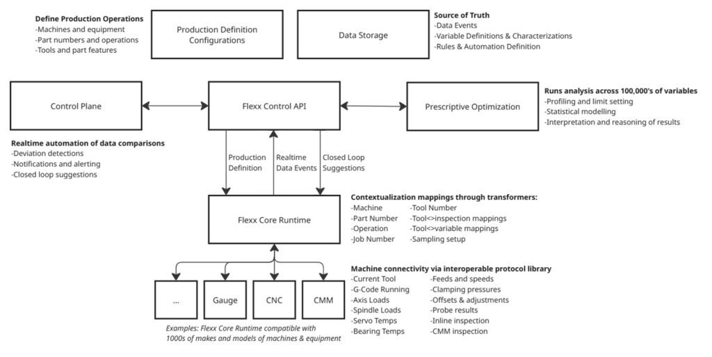
Architectural representation of the building blocks for making real-time profile deviation analysis work. 

The data needed to prevent many machining problems is already inside the CNC controller. The opportunity is to put that data to work before problems become scrap, downtime, or lost capacity.